前面已经介绍了扩散模型,在最后的结论里面提到一点:扩散模型往往需要多步才能生成较为满意的图像。不过现在有一种新的方式来加速(旨在通过少数迭代步骤)生成图像:一致性模型(consistency model),因此这里主要是介绍一致性模型(consistency model)基本原理以及代码实践,值得注意的是本文不会过多解释数学原理,数学原理推导可以参考:
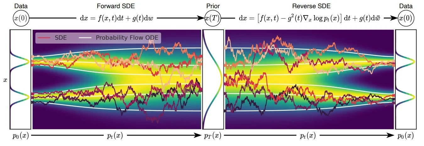
具体代码推导可以直接看最后对于LCM代码分析。介绍一致性模型之前需要了解几个知识:在传统的扩散模型中无论是加噪还是解噪过程都是随机的,在论文1中(也就是CM作者宋博士的另外一篇论文)将这个随机过程(也就是随机微分方程SDE)转化成“固定的”过程(也就是常微分方程ODE),只有过程可控才能保证下面公式成立。
一致性模型(Consistency Model)
其中
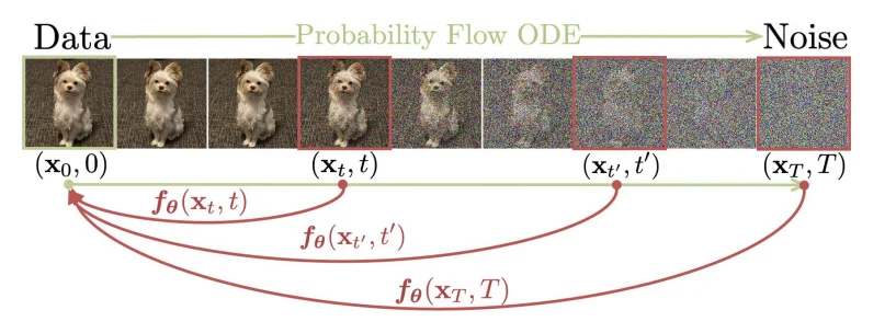
ODE(常微分方程),在传统的扩散模型(Diffusion Models, DM)中,前向过程是从原始图像 $x_0$开始,不断添加噪声,经过 $T$步得到高斯噪声图像 $x_T$。反向过程(如 DDPM)通常通过训练一个逐步去噪的模型,将 $x_T$逐步还原为 $x_0$ ,每一步估计一个中间状态,因此推理成本高(需迭代 T 步)。而在 Consistency Models(CM) 中,模型训练时引入了 Consistency Regularization,使得模型在不同的时间步 $t$都能一致地预测干净图像。这样在推理时,无需迭代多步,而是可以通过一个单一函数$f(x ,t)$ 直接将任意噪声图像$x_t$ 还原为目标图像$x_0$ 。这大大减少了推理时间,实现了一步(或少数几步)生成。
一致性模型(consistency model)在论文2里面主要是通过使用常微分方程角度出发进行解释的。Consistency Model 在 Diffusion Model 的基础上,新增了一个约束:从某个样本到某个噪声的加噪轨迹上的每一个点,都可以经过一个函数 $f$ 映射为这条轨迹的起点(也就是通过扩散处理的图像在不同的时间 $t$ 都可以直接转化为最开始的图像 $x_0$),用数学描述就是:$f:(x_t, t)\rightarrow x_\epsilon$,换言之就是需要满足: $f(x_t,t)=f(x_{t^\prime},t^\prime)$ 其中 $t,t^\prime \in [\epsilon,T]$,正如论文里面的图片描述: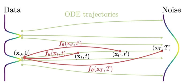
要满足上面的计算关系,作者在论文里面定义如下的等式关系(下面等式关系就是CM中核心概念):
\[f_\theta(x,t)=c_{skip}(t)x+ c_{out}(t)F_\theta(x,t)\]其中等式需要满足:$c_{skip}(\epsilon)=1,c_{out}(\epsilon)=0$ ($c_{skip}(t)=\frac{\sigma_{data}^2}{(t- \epsilon)^2+ \sigma_{data}^2}$, $c_{out}(t)=\frac{\sigma_{data}(t-\epsilon)}{\sqrt{\sigma_{data}^2+ t^2}}$),随着解噪过程(时间从:$T \rightarrow \epsilon$ 其中 $c_{skip}$ 的值逐渐增大,也就是当前的解噪图像占比权重增加),其中我的 $F_\theta$ 就是我们的神经网络模型(比如Unet)。既然使用了神经网络那么必定就需要设计一个损失函数,在论文里面作者设计的损失函数为:两个时间步之间生成得到的图像距离通过最小化这个值(比如说 $\Vert x_{t+1} - x_t \Vert_2$)来优化模型参数。作者对于模型训练给出两种训练方式
直接通过蒸馏模型进行优化
通过直接蒸馏的方式对模型参数进行优化,其中设计的损失函数为:
\[\mathcal{L}_{CD}^N(\boldsymbol{\theta},\boldsymbol{\theta}^-;\phi) = \mathbb{E}[\lambda(t_n)d(\boldsymbol{f}_{\boldsymbol{\theta}}(\mathbf{x}_{t_{n+1}},t_{n+1}),\boldsymbol{f}_{\boldsymbol{\theta}^-}(\hat{\mathbf{x}}_{t_n}^{\boldsymbol{\phi}},t_n))]\]其中 $d$代表距离(比如 $l_1$ 或者 $l_2$ )对于上面公式代表的含义是:从样本集中得到一个样本,而后加噪得到 $x_{t_{n+1}}$ ,然后利用预训练的 Diffusion 模型去一次噪,预测到另外一个点 $\hat{x}{t_n}^{\phi}$ 然后计算这两个点送入后的结果,用特定损失函数约束其一致(也就是: 模型在两个时间步之间的预测结果是否一致 也就是 $f\theta(t_{n+k})=f_\theta(t_n)$,其他的DF模型一般学的是噪声是不是一致的)。其中预测过程就是使用ODE solver进行处理,比如说:
\[\hat{x}_{t_n}^\phi= x_{t_{n+1}}- (t_n- t_{n+1})t_{n+1}\nabla_{x_{t_{n+1}}}\log p_{t_{n+1}}(x_{t_{n+1}})\]其中DDIM、DPM++就是ODE solver一种。
欧拉法: $y_{n+1}= y_n+h*f(t_n, y_n)$ 其中h代表时间步长,f代表当前导数估计。不过值得进一步了解的是,在DL中大部分函数都是直接通过神经网络进行“估算的”,也就是说对于上面的 $\nabla_{x_{t_{n+1}}}\log p_{t_{n+1}} \textcolor{red}{≈} s_\theta(x_{t_{n+1}},t_{n+1})$ 其中 $s_\theta$代表的是训练好的去噪网络。
那么这样一来整个过程就变成了: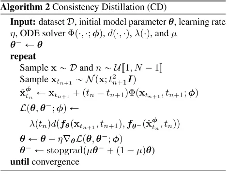
直接训练模型进行优化
直接训练模型进行优化,其中具体的过程为: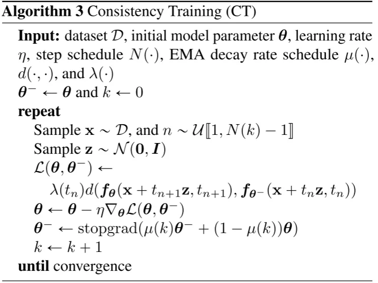
LCM/LCM-Lora
潜在一致性模型(Latent Consistency Model)3以及LCM-Lora4(LCM的Lora优微调)通过再latent space中使用一致性模型(stable diffusion model通过VAE将图像进行压缩到latent sapce而后通过DF模型训练并且最后再通过VAE decoder输出),在LCM中主要提出两点:
1、Skipping-Step:因为在最开始的CM中计算两个相邻的时间步之间的loss由于时间步过于接近,就会导致loss很小,因此通过跳步解决这个问题,这样loss就会变成:$d(f(x_{t_{n+\textcolor{red}{k}}}, t_{n+\textcolor{red}{k}}), f(x_{t_n}, t_n))$。
2、引入Classifier-free guidance (CFG) 那么整个loss计算就会变成:$d(f(x_{t_{n+\textcolor{red}{k}}}, \textcolor{red}{w}+ \textcolor{red}{c}, t_{n+\textcolor{red}{k}}), f(x_{t_n}, \textcolor{red}{w}+ \textcolor{red}{c}+ t_n))$,公式中c代表文本,对于CFG而言其实就是一个改进的ODE solver(见下面算法流程中的蓝色部分)
对于LCD算法流程,其中蓝色部分为LCM所修改的内容: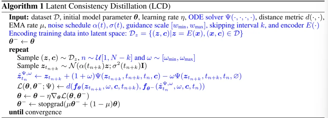
对于最后得到的实验结果分析:
- 不同的k对结果的影响
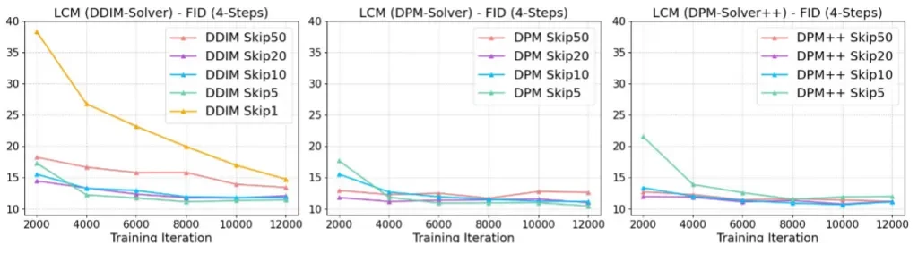
在DPM-solver++和DPM-Solver中基本只需要 2000 步迭代,LCM 4 步采样的 FID 就已经基本收敛了
- 不同的Guidance Scale对结果的影响
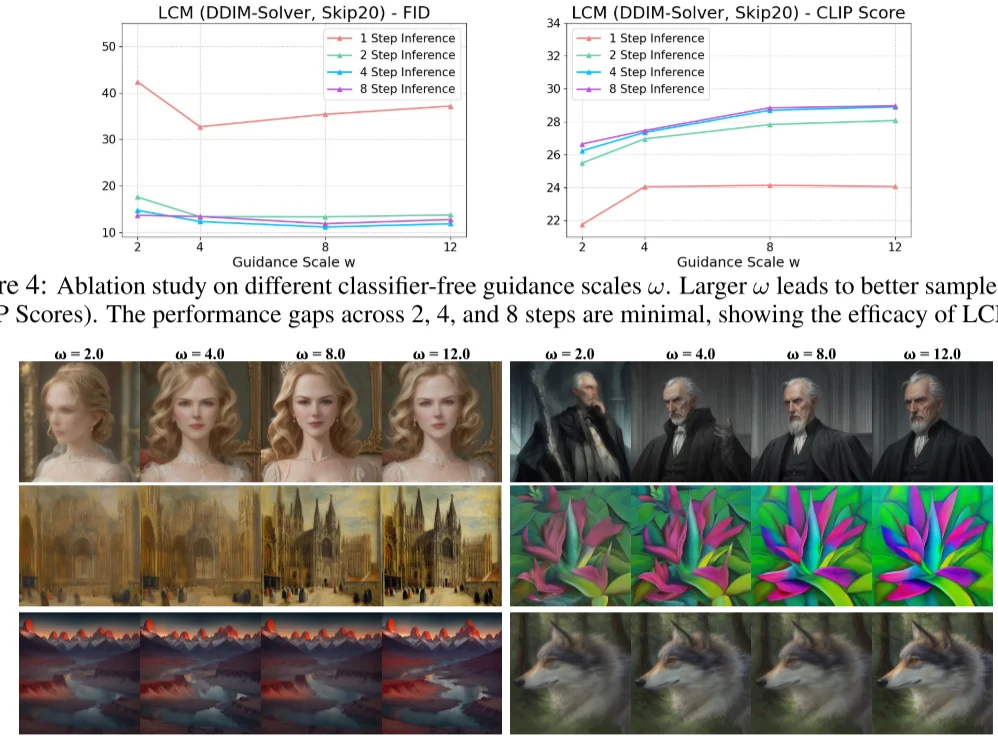
LCM 作者用不同 LCM 的迭代次数与不同 Guidance Scale 做了对比。发现 $w$ 增加有助于提升 CLIP Score,但是损失了 FID 指标(即多样性)的表现。另外,LCM 迭代次数为 2、4、8 时,CLIP Score 和 FID 相差都不大,说明了 LCM 的蒸馏性能确实非常强悍,两步前向的效果可能都足够好了,只是一步前向的结果还差些。
总得来说,在LCM中主要是做了如下几点改进:1、使用skipping-step来“拉大”相邻点之间的距离计算;2、改进了ODE solver。
LCM蒸馏训练到底在做什么?
通过结合代码理解
首先直接使用我们使用我们训练好的unet模型(unet = UNet2DConditionModel.from_pretrained)作为函数$f_\theta$。因为在CM中基于ODE(常微分方程)保证“路径”一致,并且CM核心观点就是希望模型学习从一个“晚”的时间步(接近噪声状态)预测出一个“早”的时间步(接近干净图像)下的表示(让模型学习 $z_{t_{n+k}}$ 预测出 $z_{t_n}$)。那么在采样步数过程中代码处理方式如下:
bsz = latents.shape[0]
topk = noise_scheduler.config.num_train_timesteps // args.num_ddim_timesteps #noise_scheduler使用的DDPM topk=1000//50=20 也就是说将连续时间分为 20 段
index = torch.randint(0, args.num_ddim_timesteps, (bsz,), device=latents.device).long() # 得到 t_{n+k},得到每一段的索引
start_timesteps = solver.ddim_timesteps[index] # 得到 t_{n}
timesteps = start_timesteps - topk #solver使用的DDIM
timesteps = torch.where(timesteps < 0, torch.zeros_like(timesteps), timesteps)

c_skip_start, c_out_start = scalings_for_boundary_conditions(start_timesteps,...)
...
c_skip, c_out = scalings_for_boundary_conditions(timesteps, ...)
...
noisy_model_input = noise_scheduler.add_noise(latents, noise, start_timesteps)
对于上述过程定量分析,比如说原始步骤1000步,如果蒸馏到50步LCM,那么计算步幅(topk)得到20,而后去进行随机采样(index)假设值为10,那么就可以得到起点(start_timesteps):10*20=200,终点(timesteps):200-20=180,进而计算系数在t=200时候(假设)c_skip、c_out=0.2,0.8,t=180时候c_skip、c_out=0.25,0.75。那么最终的任务中,学生模型过程拿着 $t=200$ 的噪声,试图预测 $t=0$ 的样子,教师模型过程:拿着 $t=200$ 的噪声,走一步 DDIM 到 $t=180$,告诉学生:“根据我的经验,在 $t=180$ 时图像的一致性终点应该是这个,你照着这个练。”
- 学生模型处理过程
在得到噪声之后直接输入到模型中也就是计算预测噪声(noise_pred = unet(noisy_model_input,...).sample)并且去反推预测结果 $F_\theta(x,t)$(pred_x_0 = get_predicted_original_sample()),LCM核心从某个样本到某个噪声的加噪轨迹上的每一个点,都可以经过一个函数映射为这条轨迹的起点,那么可以根据公式($f_\theta(x,t)=c_{skip}(t)x+ c_{out}(t)F_\theta(x,t)$)就可以得到(学生模型)最后的输出model_pred=c_skip_start * noisy_model_input + c_out_start * pred_x_0。也就对应下面代码:
noise = torch.randn_like(latents)
noisy_model_input = noise_scheduler.add_noise(latents, noise, start_timesteps)
...
noise_pred = unet(noisy_model_input,start_timesteps,...).sample
pred_x_0 = get_predicted_original_sample(noise_pred,start_timesteps,noisy_model_input,noise_scheduler.config.prediction_type...)#计算反推样本起点x0
model_pred = c_skip_start * noisy_model_input + c_out_start * pred_x_0
- 教师模型处理过程
处理过程和上面的处理方式是相似的(让模型学习 $z_{t_{n+k}}$ 预测出 $z_{t_n}$)也就是对应下面的:
那么具体的代码操作如下:
noisy_model_input = noise_scheduler.add_noise(latents, noise, start_timesteps)
...
accelerator.unwrap_model(unet).disable_adapters() # 因为我用lora去微调我的模型因此教师模型首先将lora取消掉
with torch.no_grad():
  # 1. Get teacher model prediction on noisy_model_input z_{t_{n + k}} and conditional embedding c
  cond_teacher_output = unet(noisy_model_input,start_timesteps,...).sample
  cond_pred_x0 = get_predicted_original_sample(cond_teacher_output,start_timesteps,noisy_model_input,...)
  cond_pred_noise = get_predicted_noise(cond_teacher_output,start_timesteps,noisy_model_input,...)

  # 2. Get teacher model prediction on noisy_model_input z_{t_{n + k}} and unconditional embedding 0
  uncond_prompt_embeds = torch.zeros_like(prompt_embeds)
  uncond_pooled_prompt_embeds = torch.zeros_like(encoded_text["text_embeds"])
  uncond_added_conditions = copy.deepcopy(encoded_text)
  uncond_added_conditions["text_embeds"] = uncond_pooled_prompt_embeds
  uncond_teacher_output = unet(noisy_model_input,start_timesteps,encoder_hidden_states=uncond_prompt_embeds.to(weight_dtype),encoder_hidden_states=uncond_prompt_embeds.to(weight_dtype),added_cond_kwargs={k: v.to(weight_dtype) for k, v in uncond_added_conditions.items()},).sample
  uncond_pred_x0 = get_predicted_original_sample(uncond_teacher_output,start_timesteps,noisy_model_input,...)
  uncond_pred_noise = get_predicted_noise(uncond_teacher_output,start_timesteps,noisy_model_input,...)

  # 3. Calculate the CFG estimate of x_0 (pred_x0) and eps_0 (pred_noise)
  pred_x0 = cond_pred_x0 + w * (cond_pred_x0 - uncond_pred_x0)
  pred_noise = cond_pred_noise + w * (cond_pred_noise - uncond_pred_noise)
  # 4. Run one step of the ODE solver to estimate the next point x_prev on the
  # augmented PF-ODE trajectory (solving backward in time)
  # Note that the DDIM step depends on both the predicted x_0 and source noise eps_0.
  x_prev = solver.ddim_step(pred_x0, pred_noise, index).to(unet.dtype)
对于上述代码可以这么理解,我的学生模型使用了Lora进行处理,我的教师模型不使用Lora处理的模型那么直接disable_adapters,在LCM的训练过程中核心思想是把输入 $x$的一部分“直接跳过” ($c_{skip}$),剩下的部分用模型预测 $F_\theta$修正,对应计算过程:$f_\theta(x,t)=c_{skip}(t)x+ c_{out}(t)F_\theta(x,t)$,那么对应学生和教师模型处理方式是一致的,只不过在LCM中会使用CFG所以处理过程就比学生模型稍复杂一点在得到预测x_0以及噪声noise之后,通过x_prev = solver.ddim_step(pred_x0, pred_noise, index)让 教师模型为学生模型提供一条确定的去噪路径(这个过程直接通过ODE计算得到),从而让学生模型学习如何从噪声生成高质量样本,而后就是计算loss:
start_timesteps = solver.ddim_timesteps[index]
timesteps = start_timesteps - topk
...
accelerator.unwrap_model(unet).enable_adapters()
with torch.no_grad():
  target_noise_pred = unet(x_prev,timesteps,...).sample
  pred_x_0 = get_predicted_original_sample(target_noise_pred,timesteps,x_prev,)
  target = c_skip * x_prev + c_out * pred_x_0

if args.loss_type == "l2":
  loss = F.mse_loss(model_pred.float(), target.float(), reduction="mean")
对于上述loss过程简单理解为:在最开始我的模型直接从200步预测最后图像并通过公式 $f_\theta(x,t)=c_{skip}(t)x+ c_{out}(t)F_\theta(x,t)$ 反推最后的结果得到model_pred,而后我的教师模型直接根据200步(start_timesteps)的加噪图像去预测噪声,并通过DDIM采样器去计算20步后的结果(180)得到 x_prev 而后我的模型再去预测180步到最后图像并且还是通过上面跳步公式得到 target,最后根据“模型在两个时间步之间的预测结果一致”假设去计算loss。
总结
总的来说在LCM中核心概念:1、从某个样本到某个噪声的加噪轨迹上的每一个点,都可以经过一个函数 $f$ 映射为这条轨迹的起点,将随机过程变为确定过程;2、模型在两个时间步之间的预测结果一致,$f(x_t,t)=f(x_{t^\prime},t^\prime)$ 其中 $t,t^\prime \in [\epsilon,T]$。除此之外为了实现少的步骤(跳步)的生成发生,通过计算公式 $f_\theta(x,t)=c_{skip}(t)x+ c_{out}(t)F_\theta(x,t)$ 直接从 $t$步跳到 $0$ 步。
训练过程可以简单理解为:对于输入图像 $x$,直接添加 $n$ 步的噪声得到 $x_n$,而后我的学生模型直接去预测 $t_0$ 时候的结果 $y_1$;同时,我的教师模型(预训练好的扩散模型)从 $x_n$ 出发,通过 DDIM 采样器向前走一步(跨越 $k$ 个时间步),得到 $t_{n-k}$ 时刻在轨迹上的观察点 $x_{n-k}$;而后再去用学生模型通过 $x_{n-k}$ 预测 $t_0$ 的结果得到 $y_2$。最后计算 $y_1$ 与 $y_2$ 之间的距离损失(Consistency Loss),迫使模型无论从哪个时间步出发,预测的终点都指向同一点。