模型量化技术
量化:是一种模型压缩的常见方法,将模型权重从高精度(如FP16或FP32)量化为低比特位(如INT8、INT4)。常见的量化策略可以分为PTQ和QAT两大类。量化感知训练(Quantization-Aware Training):在模型训练过程中进行量化,一般效果会更好一些,但需要额外训练数据和大量计算资源。后量化(Post-Training Quantization, PTQ):在模型训练完成后,对模型进行量化,无需重新训练。
因此对于量化过程总结为:将数值精度进行“校准”(比如FP32转化到INT8,两种表述范围不同,因此就需要将前者校准到后者范围),对“校准”数据进行精度转化。对于线性量化下,浮点数与定点数之间的转换公式如下:$Q=\frac{R}{S}+Z;R=(Q-Z)*S$,其中R 表示量化前的浮点数、Q 表示量化后的定点数、S(Scale)表示缩放因子的数值、Z(Zero)表示零点的数值。
量化浮点数格式:FP64、FP32、FP16、BF16等
FP以及BF之间差异就在于尾数数量上差异,除此之外在混合精度训练中也有直接使用FP16精度进行模型训练,不过FP8一般在计算过程中进行使用,模型的存储等还是使用FP16,之所以使用FP8主要还是为了节约显存加速训练,除此之外在FP8格式设计上争对不同阶段有:E4M3(表示值±448)和E5M2(表示值±57344)前面一种更加适合前向传播后面更加适合反向传播。除此之外在训练过程中使用FP8在对最后模型质量的变化差异不大1,在保证FP8训练过程中稳定:1、Per-tensor / per-block scaling(张量级 / 小块级缩放):每个权重矩阵 / 激活张量都有自己独立的缩放因子(scale),让 FP8 的动态范围“对齐”当前数据的实际分布,最大限度减少量化误差。2、Delayed scaling / delayedamax:不实时计算 scale,而是累积几步历史最大值再更新,避免 scale 抖动太大导致不稳定
模型量化具体实现过程(直接使用:https://zhuanlan.zhihu.com/p/646210009中的描述):
对称量化中,零点 Z = 0,一般不记录,我们只需要关心如何求解 Scale。由于 weight 几乎不存在异常值,因此我们可以直接取 Scale 为一个 layer 或 block 内所有参数的最大绝对值,于是所有的参数都在 [-1, 1] 的区间内。随后,这些参数将找到最近的量化格点,并转化成定点数。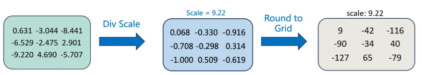
推荐进一步阅读:https://www.big-yellow-j.top/posts/2025/12/29/SDAcceralate.html
GPTQ量化技术
GPTQ2是一种用于大型语言模型(LLM)的后训练量化技术。它通过将模型权重从高精度(如FP16或FP32)压缩到低比特(如3-4位整数)来减少模型大小和内存占用,同时保持较高的推理准确性。一般而言对于量化过程为:对于给定的权重矩阵$W\in R^{n\times m}$,量化过程就是需要找到一个低比特的矩阵$\hat{W}$使得:
\[\min_{\hat{w}}\Vert WX-\hat{W}X\Vert^2_F\]其中$X$为输入向量,$\Vert. \Vert_F$为Frobenius范数。按照论文里面的描述GPTQ整个过程为: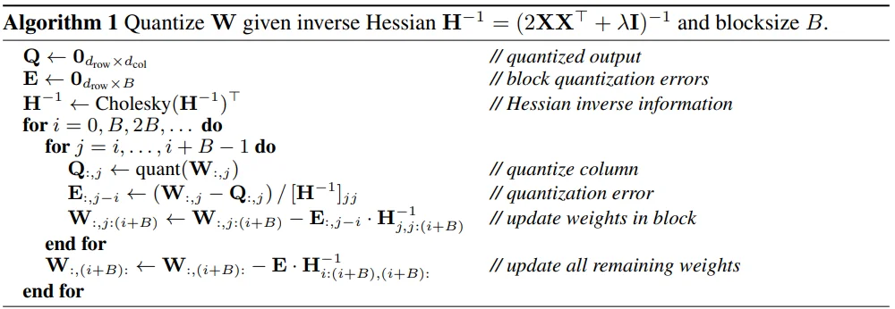
实际使用LLMCompressor进行模型量化过程中,$\lambda$对应参数
dampening_frac可能($W8A8$)会出现:Failed to invert hessian due to numerical instability. Consider increasing GPTQModifier.dampening_frac, increasing the number of calibration samples, or shuffling the calibration dataset其主要原因是计算Hessian矩阵出现严重病态(ill-conditioned)或接近奇异/非正定时,Cholesky 分解就会失败,抛出数值不稳定错误。因此就可以根据里面建议:增加数据、增加$\lambda$的值
对于具体数学原理的描述参考文章34(数学原理推荐直接看:GPTQ详细解读),简单总结一下上面过程就是:1、每行独立计算二阶海森矩阵。2、每行按顺序进行逐个参数量化,从而可以并行计算。3、按block维度进行更新,对剩余参数进行延迟更新弥补。4、对逆海森矩阵使用cholesky分解,等价消除迭代中的矩阵更新计算。它的核心流程其实就是量化-补偿-量化-补偿的迭代(具体过程见流程图中内部循环:首先量化$W_{:,j}$,而后去计算误差并且补充到 $W_{:,j:(i+B)}$),具体的代码实现过程(官方GPTQ-Github)主要是对其中LlamaAttention和LlamaMLP层中的Linear层权重进行量化。代码处理过程5:
首先、计算Hessian矩阵(因为后续计算损失和补偿权重需要,因此提前计算矩阵) 这个矩阵近似:$H_F=2X_FX_F^T$($X$是经过前面几层神经网络之后,到达被量化层的激活)。实现方式是在每一层Layer上注册hook,通过hook的方式在layer forward后使用calibration data的input来生成Hessian矩阵,这种计算方式常见于量化流程中校准数据的处理
def add_batch(name):
    def tmp(_, inp, out):
        # 假设过程为:x → Linear(W) → ReLU
        # x →inp[0].data Linear层输出→out
        gptq[name].add_batch(inp[0].data, out.data)
    return tmp
handles = []
# 添加hook
for name in subset:
    handles.append(subset[name].register_forward_hook(add_batch(name)))
# 处理样本计算数据
for j in range(args.nsamples):
    outs[j] = layer(inps[j].unsqueeze(0), attention_mask=attention_mask, position_ids=position_ids)[0]
# 去除hook
for h in handles:
    h.remove()
在add_batch中具体为了利用所有的校准数据,这里通过迭代的方式将每组数据计算的Hessian矩阵值进行求和然后取平均,代码实现是迭代逐渐平均叠加的过程,Hessian矩阵求解公式:$H_F=2X_FX_F^T$
# 假设过程为:x → Linear(W) → ReLU
# x →inp[0].data Linear层输出→out
#gptq[name].add_batch(inp[0].data, out.data)
def add_batch(self, inp, out):
    ...
    if len(inp.shape) == 2:
        inp = inp.unsqueeze(0)
    tmp = inp.shape[0]
    if isinstance(self.layer, nn.Linear) or isinstance(self.layer, transformers.Conv1D):
        if len(inp.shape) == 3:
            inp = inp.reshape((-1, inp.shape[-1]))
        inp = inp.t()
    if isinstance(self.layer, nn.Conv2d):
        unfold = nn.Unfold(
            self.layer.kernel_size,
            dilation=self.layer.dilation,
            padding=self.layer.padding,
            stride=self.layer.stride
        )
        inp = unfold(inp)
        inp = inp.permute([1, 0, 2])
        inp = inp.flatten(1)
    self.H *= self.nsamples / (self.nsamples + tmp)
    self.nsamples += tmp
    inp = math.sqrt(2 / self.nsamples) * inp.float()
    self.H += inp.matmul(inp.t())
其次、逐层weight量化
for name in subset:
    gptq[name].fasterquant(
        percdamp=args.percdamp, groupsize=args.groupsize, actorder=args.act_order, static_groups=args.static_groups
    )
    quantizers['model.layers.%d.%s' % (i, name)] = gptq[name].quantizer
    gptq[name].free()
主要是通过逐层使用fasterquant方法作为入口来进行量化处理。fasterquant 用层的权重矩阵 W 和之前收集到的激活 Gram(或近似 Hessian)H 来做按列(按 block)贪心量化。它先把 H 经过阻尼并通过 Cholesky/逆操作得到用于投影/补偿的因子(称为 Hinv),然后按 block 内逐列量化:对第 j 列量化后计算误差 e_j,用 Hinv 的相应行/列把这个误差按 Schur 补方式投影/传播到该 block 内剩余列并在 block 外一次性传播到后续列,从而实现 GPTQ 的误差补偿策略。在fasterquant方法中主要进行了量化的计算过程,具体实现过程为(核心代码):
def fasterquant(
    self, blocksize=128, percdamp=.01, groupsize=-1, actorder=False, static_groups=False
):
    W = self.layer.weight.data.clone()
    if isinstance(self.layer, nn.Conv2d):
        W = W.flatten(1)
    if isinstance(self.layer, transformers.Conv1D):
        W = W.t()
    W = W.float()

    tick = time.time()

    if not self.quantizer.ready():
        self.quantizer.find_params(W, weight=True)

    # self.H 是上一步中计算得到的Hessian矩阵
    H = self.H
    del self.H
    dead = torch.diag(H) == 0
    H[dead, dead] = 1
    W[:, dead] = 0

    ...
    # 初始化 losses 0矩阵
    Losses = torch.zeros_like(W)
    Q = torch.zeros_like(W)

    damp = percdamp * torch.mean(torch.diag(H))
    diag = torch.arange(self.columns, device=self.dev)
    H[diag, diag] += damp
    H = torch.linalg.cholesky(H)
    H = torch.cholesky_inverse(H)
    H = torch.linalg.cholesky(H, upper=True)
    Hinv = H
    # 逐Block处理
    # self.columns = W.shape[1]
    for i1 in range(0, self.columns, blocksize):
        i2 = min(i1 + blocksize, self.columns)
        count = i2 - i1

        W1 = W[:, i1:i2].clone()
        Q1 = torch.zeros_like(W1)
        Err1 = torch.zeros_like(W1)
        Losses1 = torch.zeros_like(W1)
        Hinv1 = Hinv[i1:i2, i1:i2]
        # Block内部量化
        for i in range(count):
            w = W1[:, i]
            d = Hinv1[i, i]

            if groupsize != -1:
                if not static_groups:
                    if (i1 + i) % groupsize == 0:
                        self.quantizer.find_params(W[:, (i1 + i):(i1 + i + groupsize)], weight=True)
                else:
                    idx = i1 + i
                    if actorder:
                        idx = perm[idx]
                    self.quantizer = groups[idx // groupsize]

            q = quantize(
                w.unsqueeze(1), self.quantizer.scale,
                self.quantizer.zero, self.quantizer.maxq
            ).flatten()
            Q1[:, i] = q
            Losses1[:, i] = (w - q) ** 2 / d ** 2

            err1 = (w - q) / d
            W1[:, i:] -= err1.unsqueeze(1).matmul(Hinv1[i, i:].unsqueeze(0))
            Err1[:, i] = err1

        Q[:, i1:i2] = Q1
        Losses[:, i1:i2] = Losses1 / 2

        W[:, i2:] -= Err1.matmul(Hinv[i1:i2, i2:])
    torch.cuda.synchronize()
    ...

    if actorder:
        Q = Q[:, invperm]

    if isinstance(self.layer, transformers.Conv1D):
        Q = Q.t()
    self.layer.weight.data = Q.reshape(self.layer.weight.shape).to(self.layer.weight.data.dtype)
对于上面过程主要是看两个for循环的里面内容,首先第一个for循环去根据block去将权重矩阵W进行分块拆分(W1 = W[:, i1:i2].clone()),接下来第二个for循环依次去对第1块中每列进行量化,第i列进行量化(quantize)处理(q = quantize(...)),而后去计算loss并且去对其他的列(i:)计算W1[:, i:] -= err1.unsqueeze(1).matmul(Hinv1[i, i:].unsqueeze(0)),在处理完毕第1块之后再去将后面块的列进行误差补偿(W[:, i2:] -= Err1.matmul(Hinv[i1:i2, i2:])),这样整个过程就完成了。
# 量化函数
def quantize(x, scale, zero, maxq):
    if maxq < 0:
        return (x > scale / 2).float() * scale + (x < zero / 2).float() * zero
    q = torch.clamp(torch.round(x / scale) + zero, 0, maxq)
    return scale * (q - zero)
最后、量化模型保存 。之前的步骤中量化和反量化后计算lose都是浮点位数的,所以并没有生成wbit位format的数值内容,在llama_pack方法中通过model和之前得到的quantizer(scale, zero)来生成wbit位数表达格式的量化模型,其定义如下所示
def llama_pack3(model, quantizers):
    layers = find_layers(model)
    layers = {n: layers[n] for n in quantizers}
    make_quant3(model, quantizers)
    qlayers = find_layers(model, [Quant3Linear])
    for name in qlayers:
        quantizers[name] = quantizers[name].cpu()
        # 使用 Quant3Linear 进行pack处理
        qlayers[name].pack(layers[name], quantizers[name].scale, quantizers[name].zero)
    return model
# 将model中每一层都替换为 Quant3Linear
def make_quant3(module, names, name='', faster=False):
    if isinstance(module, Quant3Linear):
        return
    for attr in dir(module):
        tmp = getattr(module, attr)
        name1 = name + '.' + attr if name != '' else attr
        if name1 in names:
            setattr(module, attr, Quant3Linear(tmp.in_features, tmp.out_features, faster=faster))
    for name1, child in module.named_children():
        make_quant3(child, names, name + '.' + name1 if name != '' else name1, faster=faster)
...
if args.wbits < 16 and not args.nearest:
    quantizers = llama_sequential(model, dataloader, DEV)
if args.save:
    llama_pack3(model, quantizers)
其中quantizers来自量化后的返回,它是一个dict里面保存了每一个层和它对应的quantizer、scale、zero、group_idx等信息,其中quantizer是layer-level的,zero和scale是group-level的。
quantizers的结果为:
quantizers['model.layers.%d.%s' % (i, name)] = (gptq[name].quantizer.cpu(), scale.cpu(), zero.cpu(), g_idx.cpu(), args.wbits, args.groupsize)
Quant3Linear具体处理过程(代码),通过qweight、zeros和scales、bias等属性来保存量化后的低比特信息。:
# qlayers[name].pack(layers[name], quantizers[name].scale, quantizers[name].zero)
class Quant3Linear(nn.Module):
    def __init__(self, infeatures, outfeatures, faster=False):
        super().__init__()
        self.register_buffer('zeros', torch.zeros((outfeatures, 1)))
        self.register_buffer('scales', torch.zeros((outfeatures, 1)))
        self.register_buffer('bias', torch.zeros(outfeatures))
        self.register_buffer(
            'qweight', torch.zeros((infeatures // 32 * 3, outfeatures), dtype=torch.int)
        )
        self.faster = faster

    def pack(self, linear, scales, zeros):
        self.zeros = zeros * scales
        self.scales = scales.clone()
        if linear.bias is not None:
            self.bias = linear.bias.clone()

        intweight = torch.round((linear.weight.data + self.zeros) / self.scales).to(torch.int)
        intweight = intweight.t().contiguous()
        intweight = intweight.numpy().astype(np.uint32)
        qweight = np.zeros(
            (intweight.shape[0] // 32 * 3, intweight.shape[1]), dtype=np.uint32
        )

        i, row = 0, 0
        while row < qweight.shape[0]:
            # 把 32 个 3-bit 整数按位连续打包到 3 个 uint32
            ...
        qweight = qweight.astype(np.int32)
        self.qweight = torch.from_numpy(qweight)
对于上述打包(3-bit打包)处理过程为:qweight = np.zeros((intweight.shape[0] // 32 * 3, intweight.shape[1]), dtype=np.uint32)每 32 个 intweight 的行使用 3 个 uint32 行来存储,不过值得注意的是以 int32 的形式存储量化权重,但这 并不代表每个权重占 32 bit。这里的 int32 是一个打包容器(bit-packing container),里面塞了多个低 bit(比如 3 bit)的权重值。
AWQ量化技术
AWQ量化6(逐层量化方法,需要每层的输入激活来计算 scale 和 clip 值)是一种基于激活值分布挑选显著权重进行量化的方法,其不依赖于任何反向传播或重建,因此可以很好地保持LLM在不同领域和模式上的泛化能力,而不会过拟合到校准集,属训练后量化大类,论文里面出发点就是模型的权重并不同等重要,仅有0.1%-1%的小部分显著权重对模型输出精度影响较大。因此如果能有办法只对0.1%~1%这一小部分权重保持原来的精度(FP16),对其他权重进行低比特量化,就可以在保持精度几乎不变的情况下,大幅降低模型内存占用,并提升推理速度。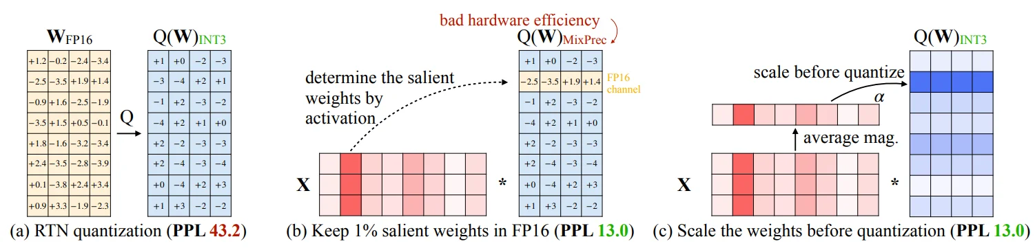
但是如果部分用FP16而其他的用INT3这样就会导致硬件上存储困难(图b情况),因此作者使用的操作就是:对所有权重均进行低比特量化,但是,在量化时,对于显著权重乘以较大的scale,相当于降低其量化误差;同时,对于非显著权重,乘以较小的scale,相当于给予更少的关注。因此代码关注点就是找到这个scale值
基于激活值分布挑选方法:激活值指的是与权重矩阵运算的输入值,比如说:$V=W_vX$其中的 $X$就是权重 $W_v$的激活值,按激活值绝对值大小由大到小排序,绝对值越大越显著,选择前0.1%~1%的元素作为显著权重。
具体代码过程(Github-Code)
首先是获取 模型第一层的输入激活值,供后续的逐层量化使用,代码整体流程如下(核心代码格式):
@torch.no_grad()
def run_awq(model,enc,w_bit,q_config,n_samples=512,seqlen=512,auto_scale=True,mse_range=True,calib_data="pileval",):
    ...

    layers = get_blocks(model)
    samples = get_calib_dataset(...)
    # 得到第一层的激活值
    inps = []
    layer_kwargs = {}

    layers[0] = layers[0].cuda()
    ...
    class Catcher(nn.Module):
        def __init__(self, module):
            super().__init__()
            self.module = module

        def forward(self, inp, **kwargs):
            inps.append(inp)
            layer_kwargs.update(kwargs)
            raise ValueError
    layers[0] = Catcher(layers[0])
    try:
        if model.__class__.__name__ == "LlavaLlamaModel":
            model.llm(samples.to(next(model.parameters()).device))
        ...
    except ValueError:
        pass
    ...
    layers[0] = layers[0].module
    inps = inps[0]
    layers[0] = layers[0].cpu()
    ...
而后、逐层进行量化处理,在AWQ量化过程中需要记录两部分量化值scale(auto_sclae.py) 和 clip(auto_clip.py)两部分具体源码处理过程都是相似的先去计算scale值而后将scale值应用,在计算两部分值之前和GPTQ处理相似去记录forward过程,具体代码为:
for i in tqdm.tqdm(range(len(layers))):
    layer = layers[i]
    layer = layer.cuda()
    named_linears = get_named_linears(layer)

    # AWQ量化过程中,记录输入数据
    def cache_input_hook(m, x, y, name, feat_dict):
        x = x[0]
        x = x.detach().cpu()
        feat_dict[name].append(x)

    input_feat = defaultdict(list)
    handles = []
    for name in named_linears:
        handles.append(
            named_linears[name].register_forward_hook(
                functools.partial(cache_input_hook, name=name, feat_dict=input_feat)
            )
        )

    inps = inps.to(next(layer.parameters()).device)
    # 输入数据被 线性层 处理触发上面的 hook 去记录每层的输入 x
    inps = layer(inps, **layer_kwargs)[0]
    for h in handles:
        h.remove()
    input_feat = {k: torch.cat(v, dim=0) for k, v in input_feat.items()}
其中cache_input_hook过程就是直接记录每层layer中的linear层的输入值并且将其记录到input_feat中。scale处理过程(寻找最有因子过程)代码如下:
elif isinstance(module, (LlamaDecoderLayer, Qwen2DecoderLayer)):
    # attention input
    scales_list.append(
        _auto_get_scale(
            prev_op=module.input_layernorm,
            layers=[
                module.self_attn.q_proj,
                module.self_attn.k_proj,
                module.self_attn.v_proj,
            ],
            inp=input_feat["self_attn.q_proj"],
            module2inspect=module.self_attn,
            kwargs=module_kwargs,
        )
    )

'''
_auto_get_scale 中核心逻辑是使用 search_module_scale 并且其中4个参数分别对应
block = module2inspect=module.self_attn
linears2scale = [module.self_attn.q_proj, module.self_attn.k_proj, module.self_attn.v_proj]
x = input_feat["self_attn.q_proj"]
'''
def _search_module_scale(block, linears2scale: list, x, kwargs={}):
    # block:对应block linears2scale:对应线性层
    x = x.to(next(block.parameters()).device)

    # 第一步,将数据数据用没有被量化的模型进行一次计算,并且计算 平均幅度(x_max)
    with torch.no_grad():
        org_out = block(x, **kwargs)
        ...
    x_max = get_act_scale(x) # x.abs().view(-1, x.shape[-1]).mean(0)

    best_error = float("inf")
    best_ratio = -1
    best_scales = None

    # 第二步,直接用网格搜索方法去寻找最优的 scale
    n_grid = 20
    history = []
    org_sd = {k: v.cpu() for k, v in block.state_dict().items()}
    for ratio in range(n_grid):
        ratio = ratio * 1 / n_grid
        # 计算当前比例的缩放因子,并且进行归一化处理
        scales = x_max.pow(ratio).clamp(min=1e-4).view(-1)
        scales = scales / (scales.max() * scales.min()).sqrt()

        # 进行一次模拟量化操作
        for fc in linears2scale:
            # 物理缩放权重:把激活值的压力转移到权重上
            fc.weight.mul_(scales.view(1, -1).to(fc.weight.device))
            # 模拟量化:量化后再除以 scales 还原回浮点域
            fc.weight.data = w_quantize_func(fc.weight.data) / (scales.view(1, -1))
        out = block(x, **kwargs) # 计算量化后的模型输出
        ...
        loss = ((org_out - out).float().pow(2).mean().item()) # 计算损失
        is_best = loss < best_error
        if is_best:
            ...
            best_scales = scales
        # 恢复到最初状态,去寻找下一个 ratio
        block.load_state_dict(org_sd)
    ...
    best_scales = best_scales.view(-1)
    ...
    return best_scales.detach()
对所有权重均进行低比特量化,但是,在量化时,对于显著权重乘以较大的scale,相当于降低其量化误差;同时,对于非显著权重,乘以较小的scale,相当于给予更少的关注
其实对于上面过程就是直接通过网格搜索策略通过得到的x_max=x.abs().view(-1, x.shape[-1]).mean(0)去不断尝试scales去让loss最小,从而得到scale值。对于其中的量化处理过程w_quantize_func,核心是计算 $q=clip(round(\frac{w}{s})+z,q_{min},q_{max})$:
'''
w_quantize_func(fc.weight.data) / (scales.view(1, -1))
w 对应 fc.weight.data) / (scales.view(1, -1)
'''
def pseudo_quantize_tensor(w, n_bit=8, zero_point=True, q_group_size=-1, inplace=False, get_scale_zp=False):
    org_w_shape = w.shape
    if q_group_size > 0:
        assert org_w_shape[-1] % q_group_size == 0
        w = w.reshape(-1, q_group_size)
    assert w.dim() == 2
    if zero_point:
        max_val = w.amax(dim=1, keepdim=True)
        min_val = w.amin(dim=1, keepdim=True)
        max_int = 2**n_bit - 1
        min_int = 0
        scales = (max_val - min_val).clamp(min=1e-5) / max_int
        zeros = (-torch.round(min_val / scales)).clamp_(min_int, max_int)
    else:  ... # 对称量化
    ...
    if inplace:...
    else:
        w = (
            torch.clamp(torch.round(w / scales) + zeros, min_int, max_int) - zeros
        ) * scales
    assert torch.isnan(w).sum() == 0
    w = w.reshape(org_w_shape)
    if get_scale_zp:...
    else:
        return w
对于上面过程总结就是:把 w 线性映射到一个由 bit 位数(n_bit)决定的固定整数区间(q_min 到 q_max),其中scale 决定缩放比例,zero_point 决定映射偏移
总结
GPTQ量化技术总结:核心流程其实就是量化-补偿-量化-补偿的迭代,首先通过对模型权重$W$首先去对$W$进行分块拆分得到不同的block再去到每一个block里面去按照每i列进行量化(quantize)处理(q = quantize(...)),而后去计算loss并且去对其他的列(i:)计算W1[:, i:] -= err1.unsqueeze(1).matmul(Hinv1[i, i:].unsqueeze(0)),在处理完毕第1块之后再去将后面块的列进行误差补偿(W[:, i2:] -= Err1.matmul(Hinv[i1:i2, i2:])),这样就得到了scales, zeros这信息,在去使用这些信息去对模型权重进行转化intweight = torch.round((linear.weight.data + self.zeros) / self.scales).to(torch.int),最后就是用32 个intweight的行使用 3 个 uint32 行来存储,推理过程的话:$y = Wx + b\rightarrow y≈x(s_j(q-z_j))+b$
AWQ量化技术总结:核心流程就是对所有权重均进行低比特量化,但是,在量化时,对于显著权重乘以较大的scale,相当于降低其量化误差;同时,对于非显著权重,乘以较小的scale,相当于给予更少的关注,对于这个scale值的寻找直接计算每一层的输入“激活值”(x.abs().view(-1, x.shape[-1]).mean(0))而后对这个激活值通过网格搜索方法(scales = x_max.pow(ratio).clamp(min=1e-4).view(-1)其中ratio对应网格收缩)不断去尝试不同的scale,并且将这个scale去用到最初的模型权重上进行一次模拟量化处理,而后去计算 模拟量化后模型计算得到的损失和没有量化的模型之间损失,找到这个最佳scale即可。
代码操作
直接使用llmcompressor来量化模型(具体地址:llmcompressor)支持量化类型: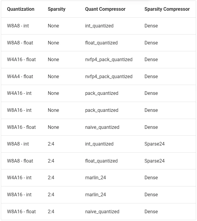
推荐进一步阅读:https://www.big-yellow-j.top/posts/2025/12/29/SDAcceralate.html